Designing a TPU and Optimizing Transformer Inference on a $100 FPGA

Designing my own TPU for transformer inference and making it go brr

This was a summer project I made to learn the basics of ML performance optimization and hardware-software co-design. The overall goal of this project is to run a small transformer on my Cmod A7 FPGA board. Then, I want to derive some of the common results you’ll find in LLM scaling (limited to a single device for now), and optimize my kernels to see how much performance I can squeeze out of my hardware design. I’m assuming you have basic knowledge on how transformer inference works (prefill, decode), but not the hardware side of things. All the code can be found in the project’s github repo .

Much of the analysis I do (including the next section), along with the TPU architecture itself, is heavily inspired by the Scaling Book . If you find this article interesting, you might enjoy reading the scaling book!

What determines how fast our model is?

Before we get into hardware, we need to ask a seemingly obvious question: what makes a model/algorithm faster? In ML, this problem can be analyzed in 2 domains: compute and communications. Compute is how many raw operations we can do in some amount of time. For example, FLOP/s (floating point operations / sec) is a common metric for the compute capabilities of GPUs or other ML accelerators. So the total compute time of an algorithm can be calculated using \(T_{\text{compute}} = \frac{\text{Total FLOPs}}{\text{Accelerator FLOPs/s}}\).

On the other hand, we have communication. In single-device inference, this usually refers to the comms between the memory (HBM, DDR) and the accelerator’s cache. In distributed inference, the comms between devices must also be considered. Similarly, if we know the memory bandwidth of our HBM or DDR, we can calculate our comms time as \(T_{\text{comms}} = \frac{\text{Communication Bytes}}{\text{Memory Bytes/sec}}\)

In most hardware, we assume that comms and compute run at the same time, so optimally, they are completely overlapped. So, our lower bound on the runtime of an algorithm is \(\max(T_{\text{comms}}, T_{\text{compute}})\). Generally speaking, our goal in designing both hardware and kernels is to analyze the bottleneck between these two and optimize it. For example, it wouldn’t make sense to try to speed up a memory-bound algorithm by trying to use more arithmetic units!

Matmuls have a special property regarding compute and comms that makes them the backbone of ML. First, let us consider an \(N\times N\times N\) matmul, in int8 (our design uses int4, but int8 keeps the byte counts clean): \(A[N, N] \cdot B[N, N] = C[N, N]\). In the best case, we have to load \(2N^2\) bytes to our compute, then write back \(N^2\) bytes to memory, which is a total of \(3N^2\). For compute, we have to perform \(N^3\) int8 multiplications. So the total arithmetic intensity of the algorithm is on the order of N, meaning it is more compute-demanding the larger our matmul gets. This is partly why matmuls are so essential to ML workloads: it is very easy to scale up our models by just throwing more compute at it to achieve larger matmuls.

Model Architecture / Goal

The overall goal is to run a transformer model on our design, while not making it completely fixed to a single architecture. We want to be able to write code to change the model architecture/dimensions, tweak our matmuls to be more efficient, or run unit tests to benchmark single layers or matmuls. This means that having fixed control flow set in hardware is not acceptable.

We will train our model and run inference on predicting the next token in an addition sequence with a maximum of 31 digits per input (64 token prefill and 64 token decode overall), which is a pretty simple but nontrivial task.

For benchmarking, we use a standard Transformer architecture, with embedding dim \(d=128\), ffn dim \(d_{ff}=512\), 4 QKV heads, and 4 layers. However, we greatly simplify some operations to allow for ease of implementation. First, we replace gelu with relu activation. Softmax in attention is also replaced with a ReLU, which makes training much harder to converge but is fine for our task. LayerNorm is replaced with a hardtanh normalization. Finally, we train with no bias in the ffn. While these are pretty major simplifications, the overall architecture stays the same, and the original goal of analyzing transformer inference performance can still be achieved.

In a transformer, we have 2 types of operations: matmuls, and elementwise ops like tensor addition and ReLU. The purpose of an accelerator is to load tensors from memory, do those operations, and write back the results. To make the most of our FPGA resources and memory, we choose to quantize activations and weights to int4.

The memory hierarchy of our TPU is simple. We are using a Cmod A7 board, which includes an Artix-7 FPGA chip along with an external asynchronous SRAM chip (8 bit read, 10 ns access time). We use the SRAM chip to model our accelerator’s external memory (HBM/DDR in a real accelerator), and the Artix-7’s BRAM to act as an on-chip cache (scratchpad memory).

There are 3 main units: MXU, VPU, and DMA. The MXU (matrix multiply unit) handles the matrix multiplications, VPU (vector processing unit) handles vector operations such as activations and addition. Both units read from the scratchpad memory and write their results back to scratchpad. The DMA (direct memory access) handles transfers between scratchpad and external memory. Each unit is controlled by a softcore PicoRV32 processor, for which we can write C firmware to dispatch instructions to each unit through AXI-based MMIO.

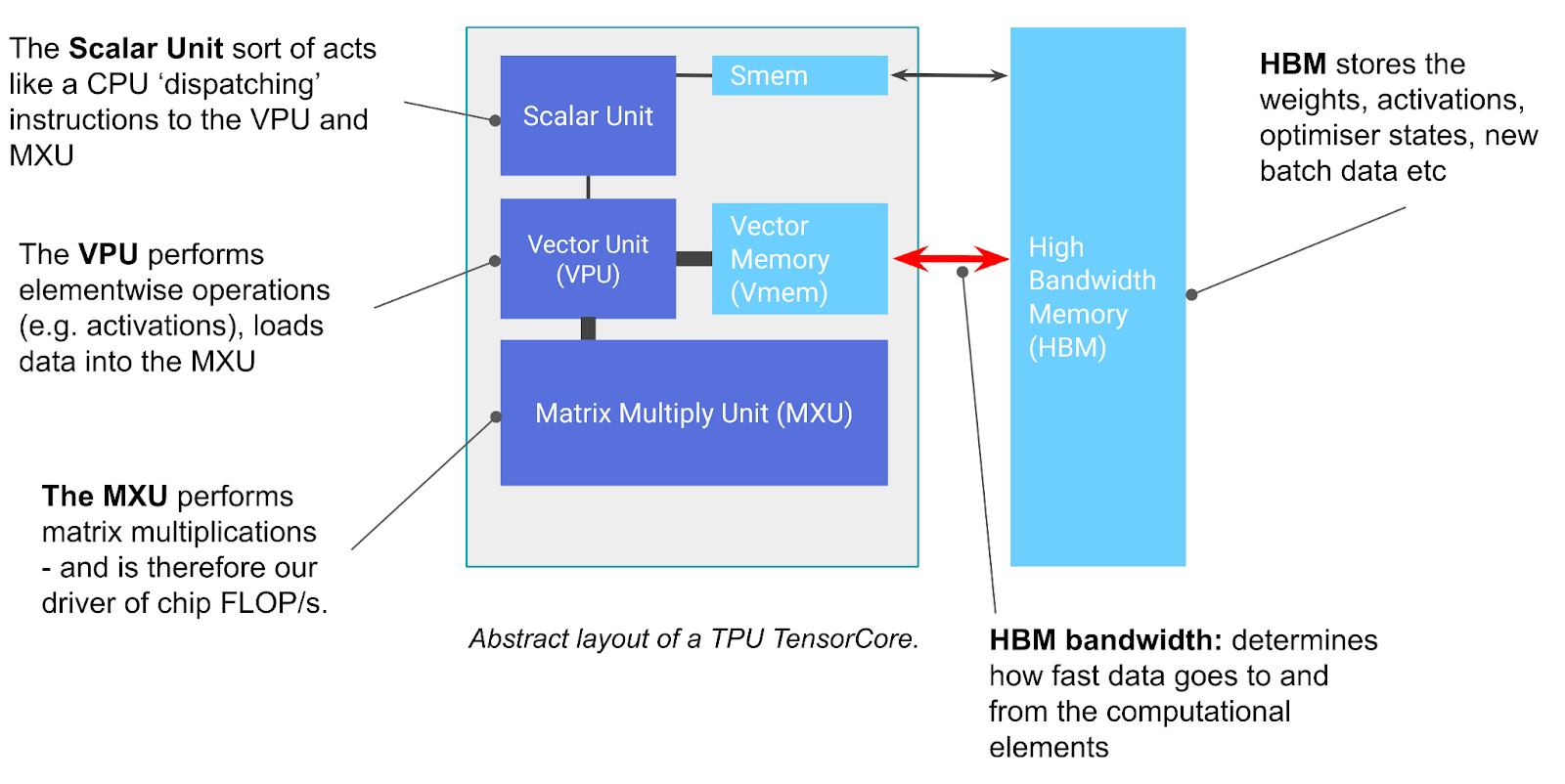
Abstract layout of a real TPU TensorCore, whose shape ours follows. Source: How To Scale Your Model

There are a few differences in our design. Vmem is our scratchpad, and HBM is our external SRAM chip. The scalar unit is just the PicoRV32 core. We also have a DMA unit, which is what actually moves data between the SRAM and the scratchpad.

Our scratchpad memory is synthesized as simple dual-port BRAM, with 2 independent ports: read and write. Since it can be synthesized to basically an arbitrary bus width for our usage (1 x 32K bits to 72 x 512 bits), we don’t need the blocks to be traditional banks indexed by address % bus_width . Instead, we can use a single block to represent a contiguous region of our scratchpad memory. This basically allows us to have as many ports accessing scratchpad as we want, with the limitation that 2 ports don’t access the same region; this will be very useful in the design later.

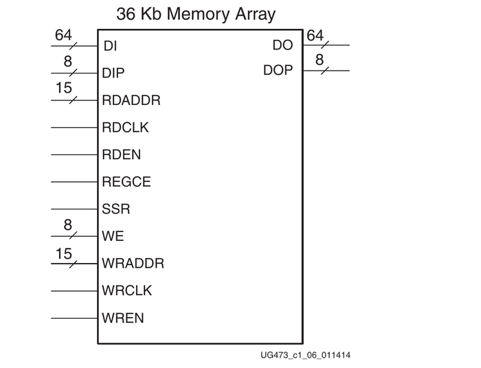
A 7-series block RAM in simple dual-port mode: one read port and one write port over the same 36 Kb array. Source: Xilinx UG473, 7 Series FPGAs Memory Resources

Our DMA is very simple. Running at the Cmod A7’s standard 12 MHz clock, the 10 ns external RAM access time is basically instant; it arrives at the next clock. The DMA unit takes in a base address for scratchpad and external RAM, a row stride, and 2d matrix dimensions, and simply drives the ports of the external RAM and scratchpad to transfer data between them. However, there is one wrinkle: since our external SRAM is asynchronous and has a 10 ns access time, the WE (write-enable) signal needs to come only after the address and data signals have arrived and stabilized. This means that for each byte written, we need to turn WE on and back off again, at the negative edge of our clock. So our final bandwidth is 1 byte / clock for external -> scratchpad, and 0.5 byte / clock for scratchpad -> external.

For matmuls, we use an output-stationary 8x8 systolic array; each PE keeps its partial sum, while moving its input values to the next PE to its right and below it. This allows us to perform an arbitrary 8xNx8 (\(A[8,N] \cdot B[N,8]\)) matmul, as long as A and B fit in scratchpad. By default, all tensors are stored row-major in both external memory and scratchpad. Since our design has no fast way to transpose a matrix, we instead use a trick in the MXU to perform transposed matmuls such as \(QK^T\) in attention. By default, A and B are fed into the systolic array like this:

2x2 version of the MXU; the real one is 8x8. Each PE stores one output element \(c_{ij}\). Left, no transpose: row \(i\) of A (blue) is loaded into that row’s register as one contiguous chunk and shifts out one element per clock. A whole B row arrives at once, and registers skew the incoming data. Right, transposed: B is stored \([N, K]\) instead, so a column’s elements are contiguous and B is fed the same way as A. This makes it so that transposed matrices never need to be re-arranged in memory; the MXU just reads them differently.

As a result, every clock, the systolic array reads \(32\) bits (8 int4 values) for matrix A and \(32\) bits for matrix B. This is where the scratchpad architecture comes in handy: as long as A and B are in different memory regions, they can be read at the same time, without interfering with ongoing DMA operations. With all \(64\) PEs accumulating one product each clock, our MXU does \(64\) multiply-accumulates per clock, which is the compute number we will use for the rest of this article.

The VPU is pretty simple. Its inputs are the base address of a vector and the length of the operation. It repeatedly loads chunks of the vector from scratchpad, operates on them (add, relu, etc.), and writes them back, until the operation is completed.

Design Choices & Other Notes

We use PicoRV32 so that we can easily write firmware for different architectures. Not only does this allow for unit testing beyond just inference and different architectures, it allows us to easily experiment with optimizations later on without having to change the dataflow in hardware.

CPU issue overhead was also a concern when designing the architecture. When the CPU dispatches instructions, they enter a command queue for each unit, which are then executed asynchronously from the CPU execution order. For synchronization, the CPU can also poll each instruction queue’s state. Furthermore, to minimize the effect of execution latency, the TPU operations are intentionally complex, allowing for instructions to span across large address ranges without needing more CPU dispatch calls.

Firmware & Kernels

We now need to program the PicoRV32 core to perform inference. First, we define our programming scheme:

We start by implementing the basic instruction dispatch to the TPU. After that, we implement primitives, namely matmul and elementwise functions.

Optimizing A Matmul

We are lucky enough to have a relatively big scratchpad (64 KB) compared to our external SRAM (512 KB), which is a 1:8 ratio. With d=128, d_ff=512, and T=64 during prefill, our largest matmul, in the FFN, requires about \((128 * 512 + 64 * 128 + 64 * 512) / 2 = 53,248\) bytes (52 KB), which can fit entirely in our scratchpad! This means that for the matmuls in our benchmark, we can basically always achieve the theoretical \(NM + MK + NK\) byte loads, since we don’t need to load the same chunk of a matrix twice when tiling.

We implement matmul as a tiled matmul over \(8\times 8\) tiles in the output matrix. Here’s the pseudocode for this kernel:

inputs (in external memory): A[M, K], B[K, N] output (in external memory): C[M, N] allocate A_tile[8*S, K], B_tile[K, 8], C_tile[8, 8] in scratchpad, in different regions. (Fit S such that it is maximized without overflowing the scratchpad.) for i from 0 to M, with step 8*S: copy A[i:i+8*S][:] from external memory to A_tile for j from 0 to N, with step 8: copy B[:][j:j+8] from external memory to B_tile wait for all DMA to finish for k from 0 to 8*S, with step 8: tpu_matmul A_tile * B_tile -> C_tile wait for mxu to finish copy C_tile from scratchpad to C[i:i+8][j:j+8] And if we instead want \(C = AB^T\), we instead load B[j:j+8][:] to B_tile, and dispatch a transpose flag when calling the mxu.

This algorithm uses less scratchpad memory than the upper bound we just calculated, and it also supports matmuls that don’t fully fit in the scratchpad by autofitting the S variable. However, in that case we lose the property above, since each element of B would have to be loaded more than once.

But this still isn’t optimal! Remember that, optimally, our runtime is the max of the MXU and DMA time. We need a way to overlap our DMA accesses with the MXU. To do this, we instead allocate 2 regions for B_tile in scratchpad, allowing us to double-buffer our DMA loads. So as our MXU is active in the k loop, we are loading the next chunk of B simultaneously, to the inactive B buffer. We will discuss the results of each optimization we do in detail later.

Optimizing Full Inference

Aside from our matmul, we also implement elementwise operations. This is pretty simple; just copy the tensor(s) to scratchpad, dispatch the VPU on the addresses, and write back to external memory. If the tensor doesn’t fit entirely, load chunks of it into scratchpad and do it multiple times.

We are now ready to implement a full inference kernel! Using our model architecture, a full prefill, for a single layer, looks like this:

model params: embedding dim d, # heads (heads), head dim d_h = d/heads inputs (in external memory, repeated for each layer): query tokens S, key/value tokens T attention weights W_Q/K/V/O[d, d], FFN weights W_1[d, 4d], W_2[4d, d].token embeddings X[T, d].outputs (in external memory, repeated for each layer): KV cache [T, 2d].for each layer: Q[S, d] = tpu_matmul(X, W_Q) K[T, d] = tpu_matmul(X, W_K) // directly at respective KV cache address V[T, d] = tpu_matmul(X, W_V) // O[S, d] = empty vector for h from 0 to heads-1: P[S, T] = tpu_matmul.transposed(Q[:][h * d_h +: d_h], K[:][h * d_h +: d_h]) P = P + mask P = relu(P) O[:][h * d_h +: d_h] = P @ V[:][h * d_h +: d_h] O = tpu_matmul(O, W_O) O = O + X O = hardtanh(O) A[S, 4d] = tpu_matmul(O, W_1) A = relu(A) Y[S, d] = tpu_matmul(A, W_2) Y = Y + O X = hardtanh(Y) In prefill, S=T.

Decode is just a special case of this, where S=1, and the K/V matrices are loaded from the KV cache instead of being recomputed every step.Let’s run a full inference, with prefill and decode:

base: run 57695827 clocks 4807.986 ms @ 12 MHz MXU busy 9752832 16.9% VPU busy 483616 0.8% DMA busy 32695968 56.7% no unit busy (issue overhead) 14763411 25.6% producer stalled on a full queue 0 0.0% two or more units busy 0 0.0% double buffered: run 47183187 clocks 3931.932 ms @ 12 MHz MXU busy 9752832 20.7% VPU busy 483616 1.0% DMA busy 32695968 69.3% no unit busy (issue overhead) 12714599 26.9% producer stalled on a full queue 0 0.0% two or more units busy 8463828 17.9% And with just prefill:

base: run 3719516 clocks 309.960 ms @ 12 MHz MXU busy 1097010 29.5% VPU busy 242200 6.5% DMA busy 2016984 54.2% no unit busy (issue overhead) 363322 9.8% producer stalled on a full queue 0 0.0% two or more units busy 0 0.0% double buffered: run 3372036 clocks 281.003 ms @ 12 MHz MXU busy 1097010 32.5% VPU busy 242200 7.2% DMA busy 2016984 59.8% no unit busy (issue overhead) 383315 11.4% producer stalled on a full queue 0 0.0% two or more units busy 367473 10.9% We see that the double buffering helps a lot! It improves our runtime by about 18% in full inference and 9% in prefill. Obviously, we haven’t achieved full overlap between compute and comms, but this is probably about as good as I could achieve without designing out-of-order execution in hardware.